Simulation

library(erglm)
library(tibble)
library(ggplot2)
theme_set(theme_bw())

Once a model has been fitted, it’s often useful to generate new data from it: for predictive checks, for simulation-based intervals, or as the input to some downstream analysis. The package offers two tools for this, operating at different levels:

simulate() is the high-level method. It generates complete replicate datasets from a fitted model, automatically propagating both the uncertainty in the parameter estimates and the observation-level noise.
erglm_fun() is the low-level building block. It extracts the deterministic prediction function from a fitted model, letting you evaluate it at any parameter values and any data you choose – the raw material for building custom simulations by hand.

Both rely on the mvtnorm package for drawing parameter values, so it needs to be installed. This article works through both tools using a gaussian model, then shows that they generalise unchanged to the other glm() families erglm supports.

mod <- erglm_model(biomarker_change ~ aucss, erglm_data, family = gaussian())

The `simulate()` method

Calling simulate() generates one or more replicate datasets. The number of replicates is set by nsim, and a seed can be supplied for reproducibility:

sim1 <- simulate(mod, nsim = 1, seed = 1)
sim1
#> # A tibble: 300 × 7
#>    dat_id sim_id     mu      val `coef_(Intercept)` coef_aucss aucss
#>     <int>  <int>  <dbl>    <dbl>              <dbl>      <dbl> <dbl>
#>  1      1      1 -0.437 -1.69                 -1.72    0.00190  673.
#>  2      2      1  3.62   6.00                 -1.72    0.00190 2806.
#>  3      3      1 -1.72  -1.22                 -1.72    0.00190    0 
#>  4      4      1  0.505 -0.722                -1.72    0.00190 1169.
#>  5      5      1 -0.999 -0.270                -1.72    0.00190  377.
#>  6      6      1 -1.09   0.00974              -1.72    0.00190  327.
#>  7      7      1 -1.72  -0.855                -1.72    0.00190    0 
#>  8      8      1  0.579  0.122                -1.72    0.00190 1208.
#>  9      9      1 -1.72   0.545                -1.72    0.00190    0 
#> 10     10      1 -1.23  -0.651                -1.72    0.00190  254.
#> # ℹ 290 more rows

What `simulate()` actually does

Generating a replicate involves two distinct sources of randomness, and simulate() accounts for both:

Parameter uncertainty. A fresh parameter vector is drawn from the multivariate normal distribution implied by the estimates and their covariance matrix, using coef(mod) and vcov(mod). This represents how uncertain we are about the fitted parameters themselves.
Observation noise. Given that parameter draw, the expected response $\mu_i$ is evaluated at each observation’s exposure and covariates, and a response is generated around it. The noise model is family-appropriate: Bernoulli draws for binomial, Poisson draws for poisson, normal draws for gaussian (as here), and gamma draws for Gamma.

Because both sources are included, the simulated val column behaves like a genuine new dataset drawn from the fitted model, not merely a noiseless prediction.

The output format

The result is a tidy, long-format tibble with nsim $\times$ nobs rows:

names(sim1)
#> [1] "dat_id"           "sim_id"           "mu"               "val"             
#> [5] "coef_(Intercept)" "coef_aucss"       "aucss"

The columns are:

dat_id – an index identifying the original observation (row of the data).
sim_id – which replicate the row belongs to (1 to nsim).
mu – the expected response (response scale) for that observation under the sampled parameters.
val – the simulated response (the mean plus family-appropriate noise).
the sampled coefficient values, prefixed coef_* (e.g. coef_`(Intercept)`, coef_aucss) to avoid colliding with predictor columns of the same name, repeated across all rows of a replicate – one parameter draw is used per replicate.
the model’s predictor columns (aucss), carried along so you can group or plot by exposure and covariates.

Requesting several replicates stacks them, and the sampled coefficients vary from one replicate to the next while staying constant within a replicate:

sims <- simulate(mod, nsim = 50, seed = 1)
dim(sims)
#> [1] 15000     7

# one parameter draw per replicate
unique(sims[sims$sim_id <= 3, c("sim_id", "coef_(Intercept)", "coef_aucss")])
#> # A tibble: 3 × 3
#>   sim_id `coef_(Intercept)` coef_aucss
#>    <int>              <dbl>      <dbl>
#> 1      1              -1.72    0.00190
#> 2      2              -1.74    0.00202
#> 3      3              -1.61    0.00176

A predictive check

A natural use of these replicates is a predictive check: if the model is adequate, the distribution of simulated responses should resemble the distribution of the observed response. Overlaying the density of the observed biomarker_change on the densities of several simulated replicates gives a quick visual check:

ggplot(sims, aes(val, group = sim_id)) +
  geom_line(stat = "density", colour = "steelblue", alpha = 0.3) +
  geom_line(
    aes(biomarker_change),
    data = erglm_data,
    stat = "density",
    inherit.aes = FALSE,
    colour = "black",
    linewidth = 1
  ) +
  labs(
    x = "Biomarker change from baseline",
    y = "Density",
    subtitle = "Observed (black) vs 50 simulated replicates (blue)"
  )

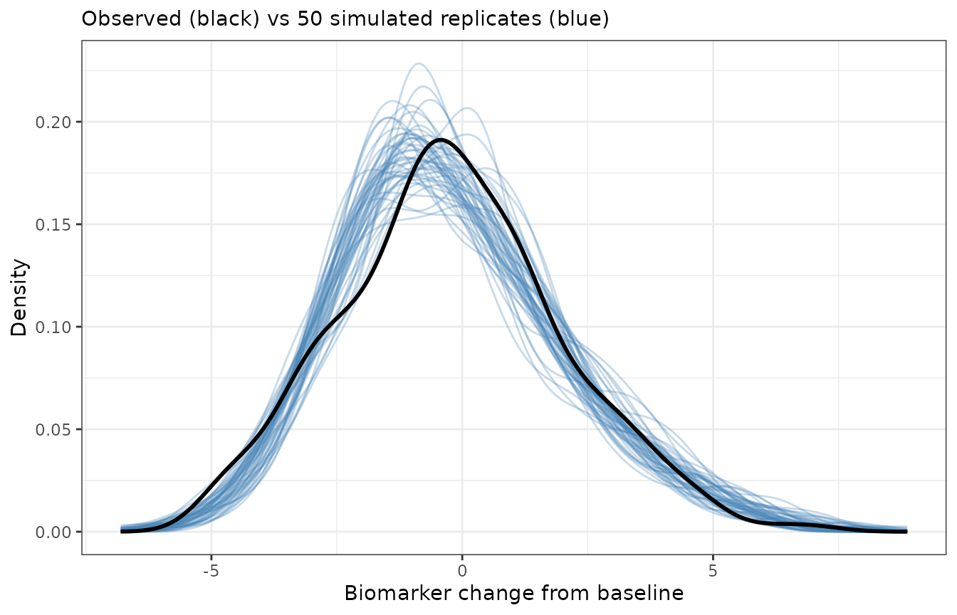
The observed distribution sits comfortably within the spread of the simulated replicates, which is what we’d hope to see from a well-fitting model.

The `erglm_fun()` tool

Where simulate() bundles parameter sampling and noise generation together, erglm_fun() exposes the deterministic core: the prediction function itself. It returns a function of two arguments, param and data, both of which default to the values used when the model was fitted:

f <- erglm_fun(mod)

# with no arguments, it reproduces the fitted values
head(f())
#> [1] -0.4013  3.5360 -1.6437  0.5142 -0.9473 -1.0400
head(fitted(mod))
#>       1       2       3       4       5       6 
#> -0.4013  3.5360 -1.6437  0.5142 -0.9473 -1.0400

Because you control both arguments, you can evaluate the model in situations the original fit never saw. Supplying param lets you ask counterfactual “what if the parameters were different?” questions – for example, setting the intercept to zero:

alt <- coef(mod)
alt["(Intercept)"] <- 0
head(f(param = alt))
#> [1] 1.2424 5.1797 0.0000 2.1579 0.6964 0.6037

Supplying data lets you evaluate the curve at exposures and covariate values of your choosing – for instance, tracing the exposure-response relationship over a grid of aucss values:

grid <- tibble(aucss = c(0, 1000, 2000, 3000, 4000))
f(data = grid)
#> [1] -1.6437  0.2022  2.0480  3.8939  5.7397

By default erglm_fun() returns predictions on the response scale (type = "response"); pass type = "link" for the link scale.

Building a custom simulation

erglm_fun() is the tool to reach for when simulate() doesn’t do exactly what you need and you want to assemble the pieces yourself. As an illustration, we can build an exposure-response curve with a parameter-uncertainty band by combining erglm_fun() with a manual parameter draw – reproducing, at a lower level, the parameter-sampling step that simulate() performs internally.

The recipe is: draw many parameter vectors from the estimated sampling distribution, evaluate the curve over an exposure grid for each draw, and summarise the resulting family of curves pointwise.

set.seed(1)
n_draws <- 500
draws <- mvtnorm::rmvnorm(n_draws, mean = coef(mod), sigma = vcov(mod))
colnames(draws) <- names(coef(mod))

curve_grid <- tibble(aucss = seq(0, max(erglm_data$aucss), length.out = 100))

# evaluate the curve for every parameter draw
curves <- apply(draws, 1, function(p) f(data = curve_grid, param = p))

# summarise pointwise across draws
band <- tibble(
  aucss = curve_grid$aucss,
  fit = f(data = curve_grid),
  lwr = apply(curves, 1, stats::quantile, probs = 0.025),
  upr = apply(curves, 1, stats::quantile, probs = 0.975)
)

ggplot(band, aes(aucss)) +
  geom_ribbon(aes(ymin = lwr, ymax = upr), fill = "firebrick", alpha = 0.2) +
  geom_line(aes(y = fit), colour = "firebrick", linewidth = 1) +
  labs(x = "AUCss", y = "Mean biomarker change", subtitle = "Point estimate with 95% parameter-uncertainty band")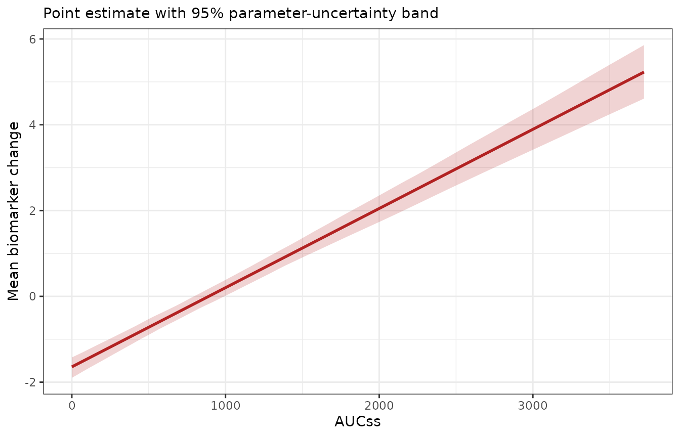

This band reflects only parameter uncertainty, because we summarised the mean curve and never added residual noise – it’s the analogue of a confidence band. Adding a step that draws rnorm(..., sd = sqrt(summary(mod)$dispersion)) around each evaluated mean would turn it into a prediction band that also captures observation noise, which is precisely the extra ingredient simulate() supplies for you. This is the essential trade-off between the two tools: simulate() is convenient and complete, while erglm_fun() is transparent and fully under your control.

The same tools across other `glm()` families

Both tools work unchanged for the other families erglm supports; only the noise model and scale differ. For a binomial model, mu is the fitted probability and val is a 0/1 outcome drawn from $\text{Bernoulli}(\mu)$ :

mod_b <- erglm_model(ae1 ~ aucss + sex, erglm_data, family = binomial())

sim_b <- simulate(mod_b, nsim = 2, seed = 1)
sort(unique(sim_b$val))
#> [1] 0 1

f_b <- erglm_fun(mod_b)
range(f_b())
#> [1] 0.1234 1.0000

For a Poisson model, val is drawn from $\text{Poisson}(\mu)$ and is always a non-negative integer:

mod_p <- erglm_model(ae_count ~ aucss + sex, erglm_data, family = poisson())

sim_p <- simulate(mod_p, nsim = 2, seed = 1)
all(sim_p$val == round(sim_p$val)) && all(sim_p$val >= 0)
#> [1] TRUE

Everything else – custom parameter values, custom data grids, and building your own simulations on top of the prediction function – carries over exactly as in the gaussian case.

Visual predictive checks

erglm_vpc_sim() is a thin, VPC-shaped wrapper around simulate(): it drops the sampled coefficients and the mu column, and splices the simulated response back into a column with the response variable’s own name, producing the data frame shape expected by erplots::er_vpc_plot():

sim <- erglm_vpc_sim(mod_b, nsim = 20, seed = 1234)
sim
#> # A tibble: 6,000 × 5
#>      ae1 aucss sex    row_id sim_id
#>    <int> <dbl> <fct>   <int>  <int>
#>  1     1  673. Male        1      1
#>  2     1 2806. Female      2      1
#>  3     1    0  Female      3      1
#>  4     1 1169. Female      4      1
#>  5     1  377. Male        5      1
#>  6     0  327. Female      6      1
#>  7     0    0  Male        7      1
#>  8     1 1208. Female      8      1
#>  9     0    0  Male        9      1
#> 10     0  254. Female     10      1
#> # ℹ 5,990 more rows

Reach for simulate() when you want the full simulation detail (sampled parameters, expected and simulated response); reach for erglm_vpc_sim() when you just want a VPC-ready data set to hand to a plotting function.

Notes

Both simulate() and erglm_fun()’s uncertainty workflows draw parameters with mvtnorm, which must be installed.
simulate() captures two sources of variability (parameter uncertainty and observation noise); a band built from erglm_fun() captures only whatever you choose to include, so decide deliberately whether you want a confidence-style band (means only) or a prediction-style band (means plus residual noise).
For a quick analytic interval on the mean, prefer erglm_predict() or predict(..., se.fit = TRUE), described in the modelling and methods articles. Reach for simulate() and erglm_fun() when you need replicate datasets or bespoke simulation logic.
Other glm() families are not currently supported by simulate()/erglm_vpc_sim() and will raise an informative error rather than silently falling back to an expectation-only draw.

The simulate() method

What simulate() actually does